SHAP

Model explainability and calculating feature SHAP values in SimBA

An understanding of how machine learning models reach their decisions is important not only for the scientific method but can also help you gain insight into how your classifier works and what makes it different or similar to other classifiers. Machine learning explainability metrics, such as SHAP, can help you answer questions like:

• Why does my classifier think some specific frames contain my behavior of interest, while other frames do not?

• Why does the classifier generated by annotator X classify events so differently (or similarly) to the classifier generated by annotator Y?

• Why does my tracking model think the location of the nose of the animal is located in this particlar part of the image?

• Which, of several classifiers, classify the target events by using the same behavioural features that a human observers would use to classify the same events?

• Are there any potential differences in the features that annotator X and annotator Y look at when annotating videos for the presence or absence of the same target behavior?

Explainability metrics can be very important, as it is possible that the classifiers you are using appear to look for the same behavioral target behaviours and features as a human observer would, while the classifier in fact looks as something very different from the human observer. Such weaknesses are typically revealed when analyzing new videos in new recording environments, that were not included in the data used to train the classifier, and explainability metrics can help you avoid those pitfalls.

Here we will look at how we can use SHAP (SHapley Additive exPlanations) within SimBA to calculate how much each feature contributes to the final behavioral classification score for each annotated video frame. Through this method we will get an verbalizable explanation for the classification probability score for each frame, such as:

Frame N in Video X was classified as containing my behavior of interest, mainly because of the distance between animal A and B, but also because the movements of animal A. In frame N, the larger movements of the animals increased the behavior classification probability with 20%, and the distance between the animals increased the classification probability with a further 70%.

In brief, when using SHAP, each feature is evaluated independently, and the final classification probability is distributed among the individual features according to their contribution to it. This value is calculated after exhaustive permutations within the order of feature-introductions into the classification scenario:

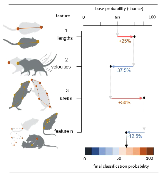
The base probability in the figure above is the probability of picking a frame that contains your behavior by pure chance (e.g., if half of your video frames contain you behavior of interest , then the base probability will be 50%; more info below!). The values associated with each feature describe the features effect on the classification probability. To read more about SHAP values, also see the SHAP GitHub repository which SimBA wraps, or read the excellent SHAP paper in Nature Machine Learning Intelligence.

Part 1: Generate a dataset

SimBA calculates SHAP values for the classifier at the same time as the model is being trained. Thus, before analysing SHAP scores, we need a dataset that contains behavioral annotations. You will need complete the steps detailed in the Scenario 1 tutorial Part 1 Step 1 up to Part 2 Step 6. That is, you will need to complete everything from Creating a project up to, and including labelling behavioral events.

Note

If you already have annotations generated elsewhere (e.g., downloaded from the SimBA OSF repository, you may not have to go through Part 1 Step 1 to Part 2 Step 6 as detailed above. When calculating the SHAP values, SimBA will loook inside your project_folder/csv/targets_inserted subdirectory for files containing the annotations (just as SimBA does when generating the classifier). So to calculate SHAP values, SimBA needs this folder to be populated with files containing behavioral annotations.

Part 2: Compute SHAP scores

Step 1: Define SHAP settings

Navigate to the Train machine model tab and click on Settings. In the pop-up window, fill out your model hyperparameter settings as described HERE. At the bottom of the Settings pop-up window, you will see these entry boxes. Begin by ticking the Calculate SHAP values entry box.

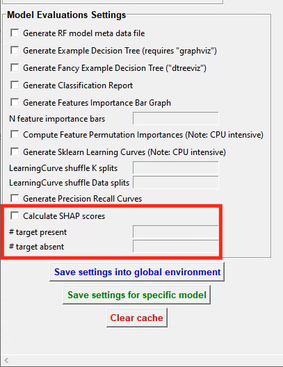
When this box is ticked, and the entry boxes are filled in, SiMBA will also calculate SHAP values while generating your behavioral classifier. SimBA will use your annotations in the project_folder/csv/targets_inserted folder when doing so. SHAP calculations are an computationally expensive process, so you most likely can’t use all of your annotations to calculate them. The time it takes to calculate SHAP scores for a single frame will depend on how many features you have the the specs of your computer, but in all likelihood it will take several seconds, and possibly tens of seconds, for a single frame. We therefore have to select a random sub-set of frames to calculate SHAP scores for.

• In the # target present entry box, enter the number of frames (integer - e.g., 200) with the behavioral target present to calculate SHAP values for.

• In the # target absent entry box, enter the number of frames (integer - e.g., 200) with the behavioral target absent to calculate SHAP values for.

Once you have filled in the SHAP entry boxes, click on either save settings into global environment or save settings for specific model, depening on wether you are generating one model, or several models at once. For more information on generating one vs several models, click HERE.

Click to close the Settings pop-up window.

Step 2: Train the classifier and generate SHAP values.

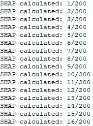
Start the classifier training by clicking on Train single model from global environment or Train multiple models, one for each saved settings. You will be able to follow the progress in the Terminal window. A new message will be printed in the main SimBA terminal for every SHAP score computed. If you are calculating the shap scores for 200 frames, you can expect the beginning of the calculations to look something like this in the main SimBA terminal:

Note

As noted above, calculating SHAP scores is computationally expensive and depending on the number of frames you entered in the # target present and # target absent, this could take a while. If you are calculating SHAP scores for a lot of frames, it’s best to make it an overnighter.

Once complete, you will see the following message: All SHAP data saved in project_folder/models/evaluations directory. Navigate to the directory to access your SHAP values. In this folder you will see two seperate CSV files. For example, if you performed SHAP calculations for a classifier called copulation, you will find the files RAW_SHAP_feature_values_copulation_prediction.csv and SHAP_values_copulation_prediction.csv. Below we will go through how the data in these two files can be interpreted.

Step 3: Interpreting the SHAP value ouput generated by SimBA.

The two SHAP value output files have an equal number of rows, where every row represent one of the frames that we calculated SHAp scores for. If you chose to generate SHAP values for 200 frames, each of the two files will contain 200 rows, where row N within both files represent the data for the same frame. The first file (SHAP_values_copulation_prediction.csv) contains the SHAP probability values. The second file (RAW_SHAP_feature_values_copulation_prediction.csv) contain the raw feature values for the same frames. The reason for generating two files is that it is sometimes necessary to match the SHAP values (represented in the SHAP_values_copulation_prediction.csv) with an actual feature values (represented in the RAW_SHAP_feature_values_copulation_prediction.csv).

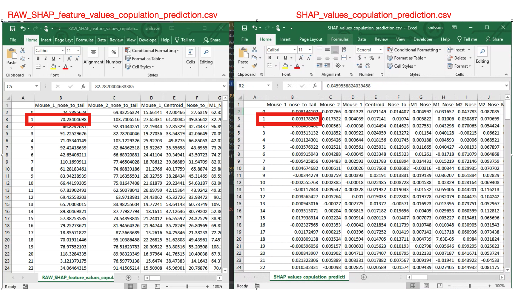
To help understand this, I’ve placed the two CSV files next to each other in the image above, with the RAW feature values file shown on the left, and the SHAP values file on the right. The red rectangle in the RAW values, on the left, shows that raw feature distance between the nose and the tail of animal number 1 (the feature name is in the header) was 70.23404 millimeters in frame number 1. Conversely, the SHAP values, shown on the right, shows that the distance between the nose and the tail of animal number 1 increased the copulation probability in frame number 1 with 0.317%.

The last four columns of the SHAP_values_copulation_prediction.csv file contain some information that might be helpful for interpretating the data, and give a sanity check that the calculations were done as expected:

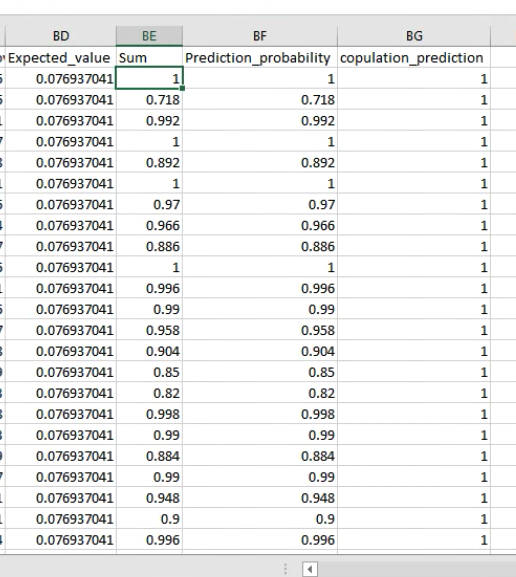
The first of these 4 columns (Expected_value), contains the baseline probability value. That is - in this toy example - if you picked a frame at random, there is a 7. 693% chance that the frame contains the target behavior copulation.

The second column (Sum) contains the sum of all of the SHAP values for each individual frame. The third column (Prediction_probability) is the classifiers probability for the presence of the behavior in each individual frame. These two columns are generated as a sanity check, because the final prediction probability seen in the `Prediction_probability` column should equal the sum of all the SHAP values seen in the `Sum` column. If the values in these two columns are not identical, then something has gone astray. Check in with us on the Gitter chat channel or raise a an issue and we may be able to help. The fourth column (copulation_prediction) will read either 0 or 1, and tell you if this particular frame was annotated as containing the behavior of interest ( 1 ), or not containing the behavior of interest ( 0 ).