Step 3: SimBA pipeline

This is a generic step by step tutorial to start using SimBA to create behavioral classifiers. For more information about the menus and options and their use cases, see the SimBA Scenario tutorials

Part 1: Create a new project

This section describes how to create a new project for your tracking analysis.

Step 1: Generate Project Config

In this step you create your main project folder with all the required sub-directories.

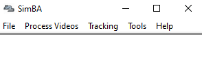
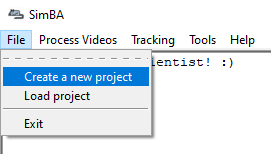
In the main SimBA window, click on File and and Create a new project. The following windows will pop up.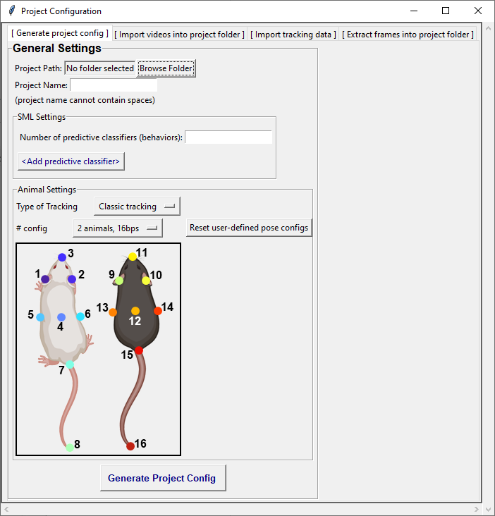
Navigate to the [ Generate project config ] tab. Under General Settings, specify a Project Path which is the directory that will contain your main project folder.
Project Name is the name of your project.

Note

Keep in mind that the project name cannot contain spaces. Instead use underscore “_”
Under SML Settings, put in the number of predictive classifiers that you wish to create. For an example, if you had three behaviors in your video, put 3 in the entry box.
Click Add Classifier and it creates a row as shown in the following image. In each entry box, fill in the name of the behavior that you want to classify.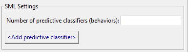
Type of Tracking allows the user to choose multi-animal tracking or the classic tracking.
Animal Settings is the number of animals and body parts that that the pose estimation tracking data contains. The default for SimBA is 2 animals and 16 body parts ( 2 animals, 16bp). There are a few other - ** yet not validated** - options, accessible in the dropdown menu.
Click on Generate Project Config to generate your project. The project folder will be located in the specified Project Path.

Step 2: Import videos into project folder

In this step, you can choose to import either one or multiple videos. The imported videos are used for visualizing predictions and standardizing distances across videos by calculating metric distances from pixel distances.

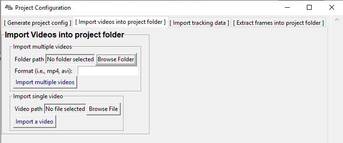
To import multiple videos

Navigate to the [ Import videos into project folder ] tab.
Under the Import multiple videos heading, click on Browse Folder to select a folder that contains all the videos that you wish to import into your project.
Enter the file type of your videos. (e.g., mp4, avi, mov, etc) in the Video type entry box.
Click on Import multiple videos.

Note

If you have a lot of videos, it might take a few minutes before all the videos are imported.

To import a single video

Under the Import single video heading, click on Browse File to select your video.
Click on Import a video.

Step 3: Import Tracking Data

In this step, you will import your pose-estimation tracking data.

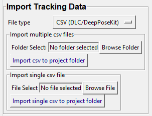
To import csv/json files

Navigate to the [ Import tracking data ] tab. Under the Import tracking data click on the File type drop down menu.
From the drop down menu, .csv files = CSV (DLC/DeepPoseKit), and .json files = JSON (BENTO).
To import multiple files, choose the folder that contains the files by clicking Browse Folder, then click Import csv to project folder.
To import a single file, choose the file by clicking Browse File, then click Import single csv to project folder.

To import h5 files (multi-animal DLC)

Please note that you can only import the h5 tracking data after you have imported the videos into the project folder.

From the File type drop down menu, select H5 (multi-animal DLC).
Under Animal settings, enter the number of animals in the videos in the No of animals entry box, and click Confirm.
Enter the names for each of the animal in the video.
Tracking type is the type of tracking from DeepLabCut multi animal tracking.
Select the folder that contains all the h5 files by clicking Browse Folder.
Click Import h5 to start importing.

To import slp files (SLEAP)

From the File type drop down menu, select SLP (SLEAP).
Under Animal settings, enter the number of animals in the videos in the No of animals entry box, and click Confirm.
Enter the names for each of the animal in the video.
Select the folder that contains all the slp files by clicking Browse Folder.
Click on Import .slp.

Step 4: Extract frames into project folder

Tip

Users no longer have to extract frames into project folder as everything will be loaded using memory and the video files.

Part 2: Load project

This section describes how to load and work with created projects.

Step 1: Load Project Config

In this step you will load the project_config.ini file that was created.

Note

A project_config.ini should always be loaded before any other process.

In the main SimBA window, click on File and Load project. The following windows will pop up.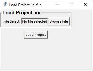
Click on Browse File. Then, go to the directory that you created your project in and click on your project folder. Locate the project_config.ini file and select it. Once this step is completed, it should look like the following, and you should no longer see the text No file selected.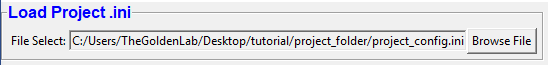

In this image, you can see the Desktop is my selected working directory, tutorial is my project name, and the last two sections of the folder path is always going to be project_folder/project_config.ini.
Click on Load Project.

Step 2 (Optional) : Import more DLC Tracking Data or videos

In this step, you can choose to import more pose estimation data in csv file format and/or more videos. If this isn’t relevant then you can skip this step.

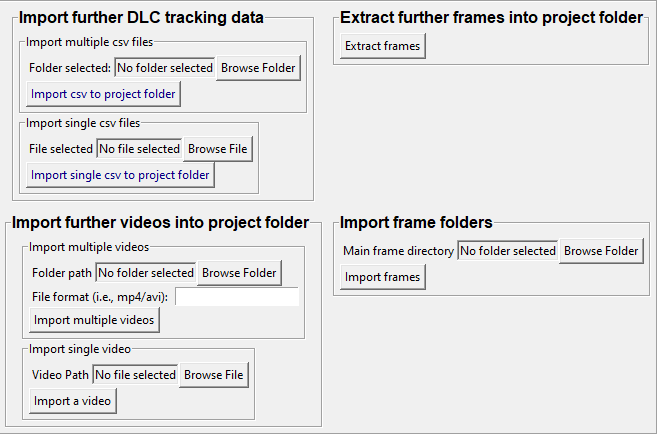
1. Click on the [ Further imports (data/video/frames) ] tab. From here you can import more data or videos into the project folder. The imported .csv files will be placed in the project_folder/csv/input directory, and the imported videos will be placed in the project_folder/videos directory.

2. Once the videos are imported, you can extract frames from the additional videos by clicking on Extract frames under the Extract further frames into project folder heading.

3. If you already have existing frames of the videos in the project folder, you can import the folder that contains the frames into the project. Under the Import frame folders heading, click on Browse Folder to choose the folder thar contains the frames, and click on Import frames. The frames will be imported into the project_folder/frames/input folder.

Step 3: Set video parameters

In this step, you can customize the meta parameters for each of your videos (fps, resolution, metric distances) and provide additional custom video information (Animal ID, group etc). You also set the pixels per millimeter for your videos. You will be using a tool that requires the known distance between two points (e.g., the cage width or the cage height) in order to calculate pixels per millimeter. The real life distance between the two points is called Distance in mm.

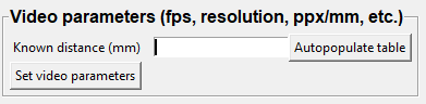
1. Under Set video parameters(distances,resolution,etc.), the entry box named Distance in mm is the known distance between two points in the videos in millimeter. If the known distance is the same in all the videos in the project, then enter the value (e.g,: 245) and click on Auto populate Distance in mm in tables. and it will auto-populate the table in the next step (see below). If you leave the Distance in mm entry box empty, the known distance will default to zero and you will fill in the value for each video individually.

Click on Set Video Parameters and the following windows will pop up.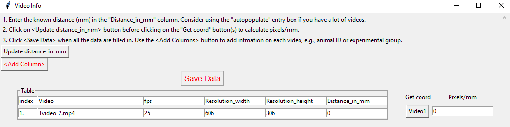

3. In the above example I imported four videos and their names are listed the leftmost Video column. I auto-populated the known distance to 10 millimeter in the previous step, and this is now displayed in the Distance in mm column.

4. I can click on the values in the entry boxes and change them until I am satisfied. Then, I click on Update distance_in_mm and this will update the whole table.

5. Next, to get the Pixels/mm for the first video, click on Video1 and the following window will pop up. The window that pops up displays the first frame of Video1.

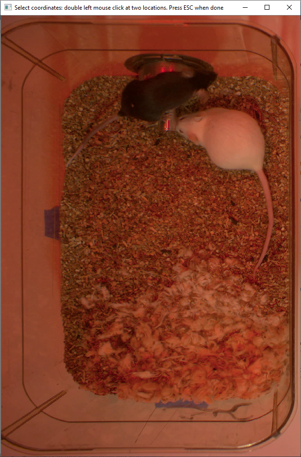
6. Now, double left click to select two points that defines the known distance in real life. In this case, I know that the two pink connected dots represent a distance of 10 millimeter in real life.

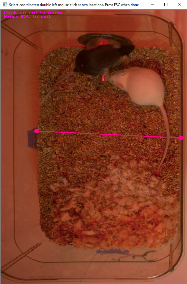
7. If you misplaced one or both of the dots, you can double click on either of the dots to place them somewhere else in the image. Once you are done, hit Esc.

8. If every step is done correctly, the Pixels/mm column in the table should populate with the number of pixels that represent one millimeter,

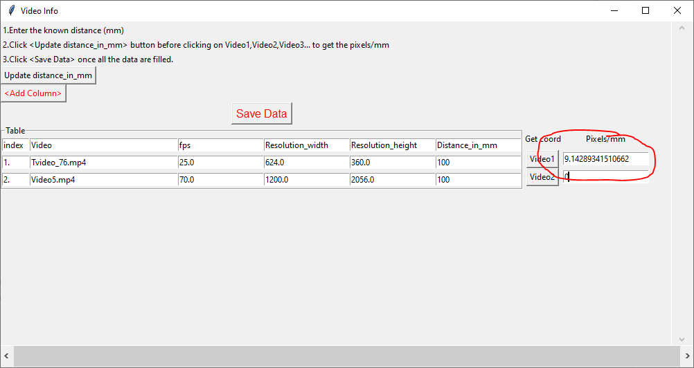
9. Repeat the steps for every video in the table, and once it is done, click on Save Data. This will generate a csv file named video_info.csv in /project_folder/log folder that contains a table with your video meta data.

10. You can also chose to add further columns to the meta data file (e.g., AnimalID or experimental group) by clicking on the Add Column button. This information will be saved in additional columns to your video_info.csv file.

Step 4: Outlier Correction

Outlier correction is used to correct gross tracking inaccuracies by detecting outliers based on movements and locations of body parts in relation to the animal body length. For more details, please click here

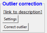
1. Click on Settings and the following window will pop up. The Outlier Settings window varies with the number of animals in the project. The images below shows settings for two animals.

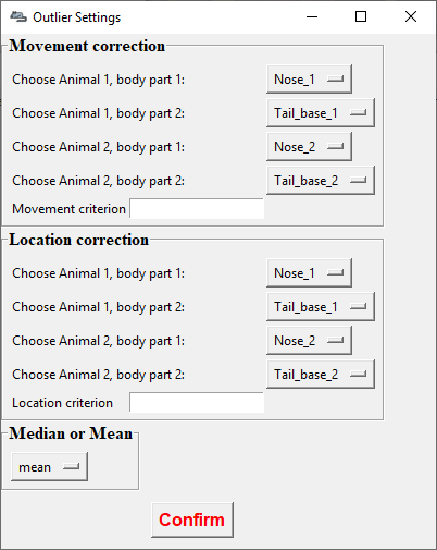
2. Select the body parts for Animal 1 and Animal 2 that you want to use to calculate a reference value. The reference value will be the mean or median Euclidian distance in millimeters between the two body parts of the two animals in all frames.

Enter values for the Movement criterion and the Location criterion.
- Movement criterion. A body part coordinate will be flagged and corrected as a “movement outlier” if the body part moves the reference value times the criterion value across two sequential frames.
- Location criterion. A body part coordinate will be flagged and correct as a “location outlier” if the distance between the body part and at least two other body parts belonging to the same animal are longer than the reference value times the criterion value within a frame.

Body parts flagged as movement or location outliers will be re-placed in their last reliable coordinate.

4. Chose to calculate the median or mean Euclidian distance in millimeters between the two body parts and click on Confirm Config.

5. Click to run the outlier correction. You can follow the progress in the main SimBA window. Once complete, two new csv log files will appear in the /project_folder/log folder. These two files contain the number of body parts corrected following the two outlier correction methods for each video in the project.

Step 5: Extract Features

Based on the coordinates of body parts in each frame - and the frame rate and the pixels per millimeter values - the feature extraction step calculates a larger set of features used for behavioral classification. Features are values such as metric distances between body parts, angles, areas, movement, paths, and their deviations and rank in individual frames and across rolling windows. This set of features will depend on the body-parts tracked during pose-estimation (which is defined when creating the project). Click here for an example list of features when tracking 2 mice and 16 body parts.

Click on Extract Features.

Step 6: Label Behavior

This step is used for label the behaviors in each frames of a video. This data will be concatenated with the features and used for creating behavioral classifiers.

There are two options, one is to start a new video annotation and one is to continue on where you last left off. Both are essentially the same, except the latter will start with the frame where you last saved. For example, one day, you started a new video by clicking Select video (create new video annotation) and you feel tired and sick of annotating the videos. You can now click Generate/Save button to save your work for your coworker to continue. Your coworker can continue by clicking ` Select folder with frames(continue existing video annotation)` and select the the video folder that you have annotated half way and take it from there!

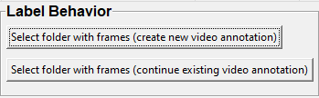
1. Click on Select video. In your project folder navigate to the /project_folder/videos/ folder, and you should select the videos that you wished to annotate.

Please click here to learn how to use the behavior annotation interface.
Once finished, click on Generate/Save and it will generate a new .csv file in /csv/targets_inserted folder.

Step 7: Train Machine Model

This step is used for training new machine models for behavioral classifications.

Note

If you import existing models, you can skip this step and go straight to Step 8 to run machine models on new video data.

Train single model

Click on Settings and the following window will pop up.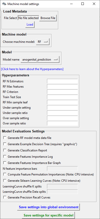

Note

If you have a .csv file containing hyper-parameter meta data, you can import this file by clicking on Browse File and then click on Load. This will autofill all the hyper-parameter entry boxes and model evaluation settings.

Under Machine Model, choose a machine model from the drop down menu: RF , GBC, XGboost.
- RF : Random forest
- GBC : Gradient boost classifier
- XGboost : eXtreme Gradient boost
Under the Model heading, use the dropdown menu to select the behavioral classifier you wish to define the hyper-parameters for.
Under Hyperparameters, select the hyper-parameter settings for your model. For more details, please click here. Alternatively, import the recommended settings from a meta data file (see above, Step 1).
- RF N estimators: Number of decision trees in the decision ensemble.
- RF Max features: Number of features to consider when looking for the best split.
- RF Criterion: The metric used to measure the quality of each split, i.e “gini” or “entropy”.
- Train Test Size: The ratio of the dataset withheld for testing the model (e.g., 0.20).
- RF Min sample leaf: The minimum number of samples required to be at a leaf node.
- Under sample setting: “Random undersample” or “None”. If “Random undersample”, a random sample of the majority class will be used in the train set. The size of this sample will be taken as a ratio of the minority class and should be specified in the “under sample ratio” box below. For more information, click here
- Under sample ratio: The ratio of samples of the majority class to the minority class in the training data set. Applied only if “Under sample setting” is set to “Random undersample”. Ignored if “Under sample setting” is set to “None” or NaN.
- Over sample setting: “SMOTE”, “SMOTEEN” or “None”. If “SMOTE” or “SMOTEEN”, synthetic data will be generated in the minority class based on k-means to balance the two classes. For more details, click here. Alternatively, import recommended settings from a meta data file (see Step 1).
- Over sample ratio: The desired ratio of the number of samples in the minority class over the number of samples in the majority class after over sampling.
Under Model Evaluation Settings.

Generate RF model meta data file: Generates a .csv file listing the hyper-parameter settings used when creating the model. The generated meta file can be used to create further models by importing it in the Load Settings menu (see above, Step 1).
Generate Example Decision Tree: Saves a visualization of a random decision tree in .pdf and .dot formats. Requires graphviz. For more information, click here
Generate Classification Report: Saves a classification report truth table in .png format. Depends on yellowbrick. For more information, click here
Generate Features Importance Log: Creates a .csv file that lists the importance’s gini importances of all features for the classifier.
Generate Features Importance Bar Graph: Creates a bar chart of the top N features based on gini importances. Specify N in the N feature importance bars entry box below.
N feature importance bars: Integer defining the number of top features to be included in the bar graph (e.g., 15).
Compute Feature Permutation Importance's: Creates a .csv file listing the importance’s (permutation importance’s) of all features for the classifier. For more details, please click here. Note: Calculating permutation importance’s is computationally expensive and takes a long time.
Generate Sklearn Learning Curve: Creates a .csv file listing the f1 score at different test data sizes. For more details, please click here. This is useful for estimating the benefit of annotating further data.
LearningCurve shuffle K splits: Number of cross validations applied at each test data size in the learning curve.
LearningCurve shuffle Data splits: Number of test data sizes in the learning curve.
Generate Precision Recall Curves: Creates a .csv file listing precision at different recall values. This is useful for titration of the false positive vs. false negative classifications of the models.

Click on the Save settings into global environment button to save your settings into the project_config.ini file and use the settings to train a single model.
Alternatively, click on the Save settings for specific model button to save the settings for one model. To generate multiple models - for either multiple different behaviors and/or using multiple different hyper-parameters - re-define the Machine model settings and click on Save settings for specific model again. Each time the Save settings for specific model is clicked, a new config file is generated in the /project_folder/configs folder. In the next step (see below), a model for each config file will be created if pressing the Train multiple models, one for each saved settings button.
If training a single model, click on Train Model.

To train multiple models

Click on Settings.
Under Machine Model, choose the machine model from the drop down menu, RF , GBC, Xboost.
Under Model, select the model you wish to train from the drop down menu.
Then, set the Hyperparameters.
Click the Save settings for specific model button. This generates a meta.csv file, located in your project_folder/configs directory, which contains your selected hyperparameters. Repeat the steps to generate multiple models. On model will be generated for each of the meta.csv files in the project_folder/configs directory.
Close the Machine models settings window.
Click on the green Train Multiple Models, one for each saved settings button.

Optional step before running machine model on new data

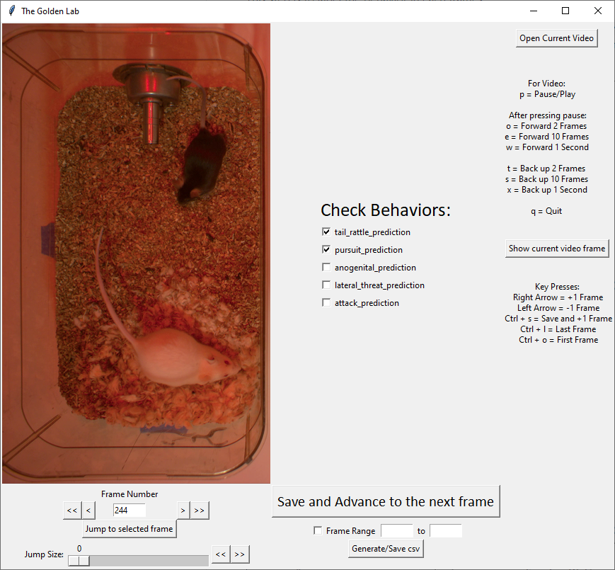
The user can validate each model ( saved in .sav format) file. In this validation step the user specifies the path to a previously created model in .sav file format, and a .csv file containing the features extracted from a video. This process will (i) run the classifications on the video, and (ii) create a video with the predictions overlaid together with a gantt plot showing predicted behavioral bouts. Click here for an example validation video.

Click Browse File and select the project_config.ini file and click Load Project.
Under [Run machine model] tab –> validate Model on Single Video, select your features file (.csv). It should be located in project_folder/csv/features_extracted.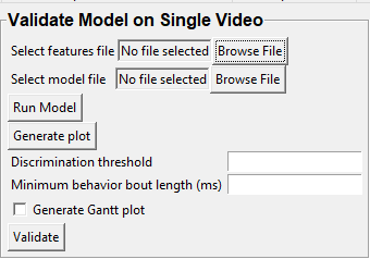
Under Select model file, click on Browse File to select a model (.sav file).
Click on Run Model.
Once, it is completed, it should print “Predictions generated.”, now you can click on Generate plot. A graph window and a frame window will pop up.
- Graph window: model prediction probability versus frame numbers will be plot. The graph is interactive, click on the graph and the frame window will display the selected frames.
- Frame window: Frames of the chosen video with controls.

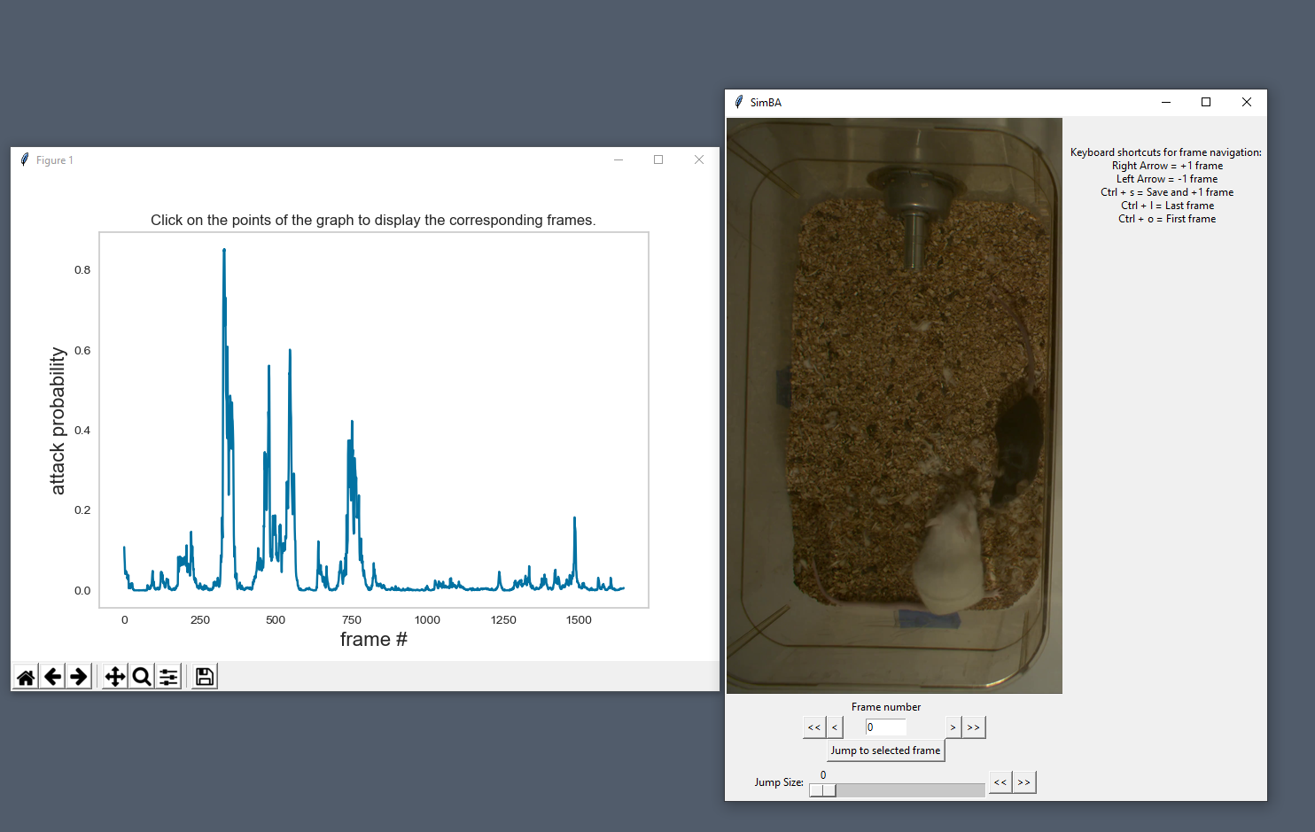
Click on the points on the graph and picture displayed on the other window will jump to the corresponding frame. There will be a red line to show the points that you have clicked.
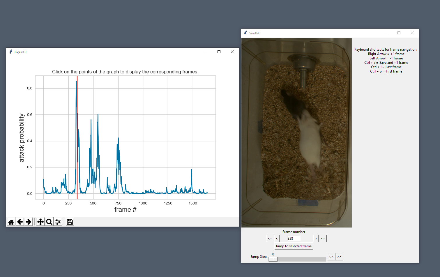
Once it jumps to the desired frame, you can navigate through the frames to determine if the behavior is present. This step is to find the optimal threshold to validate your model.
Once the threshold is determined, enter the threshold into the Discrimination threshold entry box and the desire minimum behavior bouth length into the Minimum behavior bout lenght(ms) entrybox.
- Discrimination threshold: The level of probability required to define that the frame belongs to the target class. Accepts a float value between 0.0-1.0. For example, if set to 0.50, then all frames with a probability of containing the behavior of 0.5 or above will be classified as containing the behavior. For more information on classification threshold, click here
- Minimum behavior bout length (ms): The minimum length of a classified behavioral bout. Example: The random forest makes the following attack predictions for 9 consecutive frames in a 50 fps video: 1,1,1,1,0,1,1,1,1. This would mean, if we don’t have a minimum bout length, that the animals fought for 80ms (4 frames), took a brake for 20ms (1 frame), then fought again for another 80ms (4 frames). You may want to classify this as a single 180ms attack bout rather than two separate 80ms attack bouts. With this setting you can do this. If the minimum behavior bout length is set to 20, any interruption in the behavior that is 20ms or shorter will be removed and the behavioral sequence above will be re-classified as: 1,1,1,1,1,1,1,1,1 - and instead classified as a single 180ms attack bout.
Click Validate to validate your model. Note that this step will take a long time as it will generate a lot of frames.

Step 8: Run Machine Model

This step runs behavioral classifiers on new data.

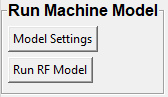
Under the Run Machine Model heading, click on Model Selection. The following window with the classifier names defined in the project_config.ini file will pop up.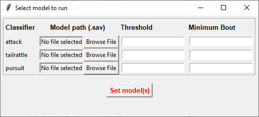
Click on Browse File and select the model (.sav) file associated with each of the classifier names.
Once all the models have been chosen, click on Set Model to save the paths.
Fill in the Discrimination threshold.
- Discrimination threshold: The level of probability required to define that the frame belongs to the target class (see above).
Fill in the Minimum behavior bout length.
- Minimum behavior bout length (ms): The minimum length of a classified behavioral bout(see above).
Click on Set model(s) and then click on Run RF Model to run the machine model on the new data.

Step 9: Analyze Machine Results

Access this menu through the Load project menu and the Run machine model tab. This step performs summary analyses and presents descriptive statistics in .csv file format. There are three forms of summary analyses: Analyze, Analyze distance/velocity, and Analyze severity.

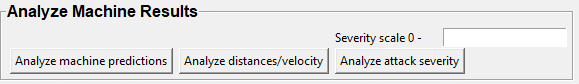
Analyze: This button generates descriptive statistics for each predictive classifier in the project, including the total time, the number of frames, total number of ‘bouts’, mean and median bout interval, time to first occurrence, and mean and median interval between each bout. A date-time stamped output csv file with the data is saved in the /project_folder/log folder.

Analyze distance/velocity: This button generates descriptive statistics for mean and median movements and distances between animals. The date-time stamped output csv file with the data is saved in the /project_folder/log folder.

Analyze severity: Calculates the ‘severity’ of each frame classified as containing attack behavior based on a user-defined scale. Example: the user sets a 10-point scale. One frame is predicted to contain an attack, and the total body-part movements of both animals in that frame is in the top 10% percentile of movements in the entire video. In this frame, the attack will be scored as a 10 on the 10-point scale. A date-time stamped output .csv file containing the ‘severity’ data is saved in the /project_folder/log folder.

Severity scale 0 -:

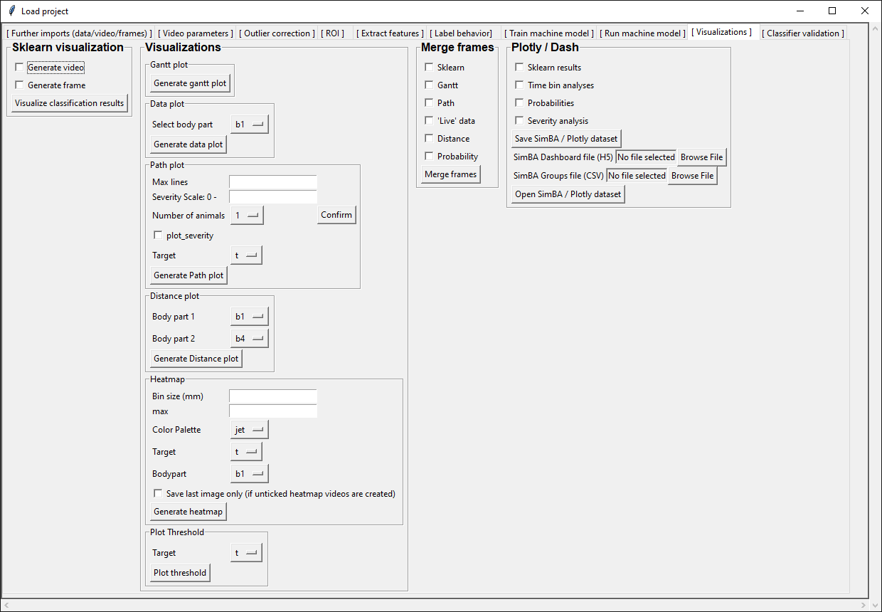
Step 10: Sklearn Visualization

These steps generate visualizations of features and machine learning classification results. This includes images and videos of the animals with prediction overlays, gantt plots, line plots, paths plots and data plots. In this step the different frames can also be merged into video mp4 format.

Under the Sklearn visualization heading, check on the box and click on Visualize classification results.
- Generate video: This generates a video of the classification result
- Generate frame: This generates frames(images) of the classification result
Note

Generate frames are required if you want to merge frames into videos in the future.

This step grabs the frames of the videos in the project, and draws circles at the location of the tracked body parts, the convex hull of the animal, and prints the behavioral predictions on top of the frame. For an example, click here

Step 11: Visualizations

The user can also create a range of plots: gantt plot, Data plot, Path plot, Distance plot, and Heatmap.

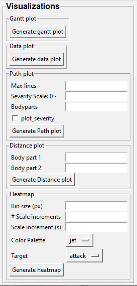
Gantt plot

Gantt plot generates gantt plots that display the length and frequencies of behavioral bouts for all the videos in the project.

Under the Gantt plot heading, click on Generate Gantt plot and gantt plot frames will be generated in the project_folder/frames/output/gantt_plots folder.

Data plot

Generates ‘live’ data plot frames for all of the videos in the project that display current distances and velocities.

Under the Data plot heading, click on Generate Data plot and data plot frames will be generated in the project_folder/frames/output/live_data_table folder.

Path plot

Generates path plots displaying the current location of the animal trajectories, and location and severity of attack behavior, for all of the videos in the project.

Under the Path plot heading, fill in the following user defined values.
- Max Lines: Integer specifying the max number of lines depicting the path of the animals. For example, if 100, the most recent 100 movements of animal 1 and animal 2 will be plotted as lines.
- Severity Scale: Integer specifying the scale on which to classify ‘severity’. For example, if set to 10, all frames containing attack behavior will be classified from 1 to 10 (see above).
- Bodyparts: String to specify the bodyparts tracked in the path plot. For example, if Nose_1 and Centroid_2, the nose of animal 1 and the centroid of animal 2 will be represented in the path plot.
- plot_severity: Tick this box to include color-coded circles on the path plot that signify the location and severity of attack interactions.
Click on Generate Path plot, and path plot frames will be generated in the project_folder/frames/output/path_plots folder.

Distance plot

Generates distance line plots between two body parts for all of the videos in the project.

Fill in the Body part 1 and Body part 2
- Body part 1: String that specifies the the bodypart of animal 1. Eg., Nose_1
- Body part 2: String that specifies the the bodypart of animal 1. Eg., Nose_2
Click on Generate Distance plot, and the distance plot frames will be generated in the project_folder/frames/output/line_plot folder.

Heatmap

Generates heatmap of behavior that happened in the video.

To generate heatmaps, SimBA needs several user-defined variables:

Bin size(mm) : Pose-estimation coupled with supervised machine learning in SimBA gives information on the location of an event at the single pixel resolution, which is too-high of a resolution to be useful in heatmap generation. In this entry box, insert an integer value (e.g., 100) that dictates, in pixels, how big a location is. For example, if the user inserts 100, and the video is filmed using 1000x1000 pixels, then SimBA will generate a heatmap based on 10x10 locations (each being 100x100 pixels large).

max (integer, or auto): How many color increments on the heatmap that should be generated. For example, if the user inputs 11, then a 11-point scale will be created (as in the gifs above). If the user inserts auto in this entry box, then SimBA will calculate the ideal number of increments automatically for each video.

Color Palette : Which color pallette to use to plot the heatmap. See the gifs above for different output examples.

Target: Which target behavior to plot in the heatmap. As the number of behavioral target events increment in a specific location, the color representing that region changes.

Bodypart: To determine the location of the event in the video, SimBA uses a single body-part coordinate. Specify which body-part to use here.

Save last image only: Users can either choose to generate a “heatmap video” for every video in your project. These videos contain one frame for every frame in your video. Alternative, users may want to generate a single image representing the final heatmap and all of the events in each video - with one png for every video in your project. If you’d like to generate single images, tick this box. If you do not tick this box, then videos will be generated (which is significantly more time-consuming).

Click Generate heatmap to generate heatmap of the target behavior. For more information on heatmaps based on behavioral events in SimBA - check the tutorial for scenario 2 - visualizing machine predictions

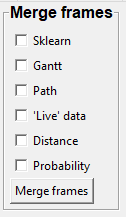
Step 12: Merge Frames

Merge all the generated plots from the previous step into a single frame and generate a video as an output.

Note

All the frames must be generated in the previous step for this to work. This step combines all the frames(images) that are generated and merge them together and make a video.**

Check on the plot that you wish to merge together and output as a single video.
Under Merge Frames, click Merge Frames and frames with all the generated plots will be combined and saved in the project_folder/frames/output/merged folder in a video format.

Plotly

Please click here to learn how to use plotly.